Aurora DSQL and the Circle of Life
In this article we’re going to take a deeper look at the Circle of Life in Aurora DSQL. Understanding the flow of data will really help you wrap your head around the DSQL architecture, and how best to build applications against DSQL.
My intention in sharing this article is help you understand the flow. There are many other things to understand: availability, scalability, durability, security, and so on. I won’t be discussing those in detail, because each of those topics is deep and complex, and deserves its own focus.
The flow of data
Aurora DSQL is based on PostgreSQL. The Query Processor (QP) component is a running postgres process, although we’ve significantly modified it to work with our architecture.
If you connect to DSQL with a Postgres client (such as psql), you’re connected
to one of these postgres processes. You’re connected to a QP, and you can start
to interact with it as you would with any other Postgres server.
If you run a local Postgres operation, such as SELECT 1, then that query is
processed entirely locally by the QP. But what happens when you query a table:
select * from test;
 id | value
----+-------
  1 |    10
(1 row)
Usually, you’d expect Postgres to read from storage locally, which might mean reading from the buffer cache, or doing disk I/O. When running on Aurora Postgres (APG), cache misses would result in a load from remote storage.
Like APG, reads in DSQL also go to remote storage. In our above query, which
is a scan of the entire test table, the QP is going to turn around and scan
storage, and storage is going to return all the rows in the table.
But how did storage get the rows in the first place?
insert into test values (1, 10); -- autocommit
Vanilla Postgres would process that transaction locally, inserting into the
Write-Ahead Log (WAL), updating the buffer cache, and using fsync() to persist
the changes to disk. In APG, the buffer cache is also updated, but the
durability of the transaction is ensured by fsync() to the remote storage in
multiple Availability Zones (AZ).
Commits in DSQL have the same basic ingredients, but they’re expressed quite differently. In DSQL, data is durably persisted when it’s written to the journal1. Storage follows the journal, and keeps itself up to date.
When I first started working on DSQL (many years ago!), I didn’t really get this flow. I’d been told “writes go to the journal, reads go to storage”. I nodded, but I didn’t deeply, truly, understand that simple explanation. I’d spent too much time with traditional architectures, and my mind kept falling back on the familiar.
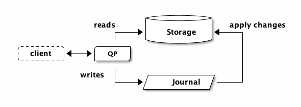
What helped me get it was the picture at the top of this post. Imagine somebody drawing this on the whiteboard. They draw the three boxes: QP, journal and storage. Then, they draw the Circle of Life:

There’s something about this presentation, vs. the one at the top of the article, that helped it go click for me. Removing the service interactions certainly helps. Notice how in the first picture there’s an arrow from the QP to storage, while in the Circle, the arrow is the other way round?
“Writes go to the journal, reads go to storage”, never quite did it for me. “Writes never go to storage, reads never go to the journal” also didn’t quite the message across. The Circle did for me, and I hope it does for you.
The flow of time
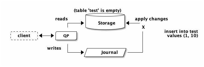
Now you may be thinking: How do we know that storage is up to date? We’ve just
inserted our (1, 100) tuple and got a successful commit. Then, we run our
table scan. What if storage isn’t up to date? What if there’s some kind of
delay on the network, preventing storage from learning about the new row?
The change is trying to reach storage, but it’s stuck in traffic:
The answer to this question is quite beautiful, and it’s one of the things I’m most excited about with DSQL. Because the answer is absolutely not “eventual consistency”.
You see, it’s not just data that’s flowing around the Circle, it’s time too.
Every transaction has a start time Tstart. This time comes from EC2 Time
Sync, which provides us with microsecond-accurate time. When the QP queries
storage, it doesn’t just ask “give me all the rows in the test table”.
Instead, it adds “.. as of Tstart”. When the QP writes data to the journal,
it computes the commit time and then says “store this data at Tcommit”.
The journal provides an ordered stream of both time and data, which means storage can know precisely when it has all the data to answer the query.
As somebody who’s spent an awful amount of time debugging and trying work around bugs caused by eventual consistency, I really cannot overstate how delighted I am with this design property. In DSQL, you never have to deal with eventual consistency. You either get:
- the right answer immediately,
- or you get the right answer with a slight delay,
- or you get an error (and we get paged).
You never get the wrong answer - you never get stale data.
And, of course, we’ve put an enormous amount of engineering effort into keeping the cases of delays as infrequent as possible even in the event of hardware or networking failures.
Implications
I’m going to share some positive implications of this architecture. In a future article, we’ll talk about some of the patterns that don’t work so well on this architecture, and what you should do instead.
It scales like crazy
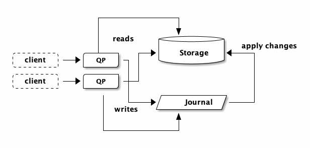
The whole point of a distributed architecture like DSQL is to enable better scalability, availability and so on (read Why do we need distributed systems?). DSQL is designed to scale horizontally. If you open a second connection to DSQL, your picture now looks like this:
If you open more connections and do more (and more) reads, DSQL will detect the increase in traffic, add more storage capacity, and now suddenly you have:
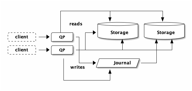
The same idea is true of the journal, and all the other DSQL architectural components that I’m not showing here. DSQL scales horizontally. If we’re running out of something, we just add more of it. We’re also able to partition data up; there’s nothing in this picture that says any of the storage boxes needs to contain all the data.
In DSQL, scaling is completely hands-free. If you’ve opened more than one connection to DSQL, you’ve already scaled out.
No eventual consistency
In DSQL, there is no eventual consistency, at any scale.
Most deployments of relational databases run into this problem. Your primary is running hot. You realize you have way more reads than writes. So you add a read replica.
But now you need to teach your application about read replicas. Which queries should go to the primary, which should go to a replica?
Then you add more replicas. How do I learn about all the replicas, how do I load balance across them?
Replicas are usually up to date, and so you might not realize how many bugs you’ve just introduced. Sooner or later, things are going to slow down, and now you need to go find all the cases where you really did need to ensure you had the latest data. If I sound like I have some eventual consistency trauma, that’s because I do.
In DSQL, you don’t have to worry about any of this. DSQL automatically manages the internal capacity for your cluster. DSQL automatically ensures your queries have fresh data.
This property goes hand-in-hand with hands-free, automatic scaling. If adding storage replicas were to introduce eventual consistency, then we couldn’t do it automatically.
But it gets even cooler than that.
No eventual consistency, even across Regions
In DSQL, there is no eventual consistency, at any scale, even when doing multi-Region.
The Circle of Life doesn’t care about being in the same AWS region. Let’s look at multi-Region. Depending on how you’re reading this article, you might want to open the next picture in a new tab:
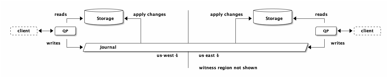
What’s really important to emphasize here is that reads are always local. If you insert data into the region on the left and then read it from the region on the right, the read in the region on the right is fast and local. The QP on the right has absolutely no clue where the data came from, nor does storage. The QP just says “hey, give me the data as of Tstart” and storage just waits until it’s seen everything and then returns the results.
Here’s the story I like to tell: imagine you have a DSQL cluster somewhere on planet Earth, and another, peered, cluster somewhere far away - say…on the Moon. On Earth, we insert some data:
insert into test values (1, 10); -- autocommit
The Internet tells me it’s about 2.5s RTT to the Moon, so expect about that much latency on commit. The spooky bit comes next. A user in either location can then run:
select * from test;
No matter whether you’re on Earth, or on the Moon, you’re going to see the inserted row (no eventual consistency), and you’re going to see it with low latency. This may seem like magic. Are we breaking the laws of physics? Not at all; the reason the commit took 2.5s was to get the data on the moon. So, by the time the astronaut runs her query, there’s no need to wait.
Summary
In this article, we’ve taken a look at how data flows through the DSQL architecture, and how this design allows for horizontal scaling without eventual consistency even across AWS regions.
I hope this article gives you some ideas for how best to use DSQL, and some intuition as to where DSQL can solve some of the problems you might be facing.
Footnotes:
In multiple AZs. For multi-Region clusters; in multiple AWS regions.